In this blog, we learn about the Auto Insurance Data and highutilize K Means clustering in Python to segment customers based on their transaction history. We will utilize these segments to futher understand customer traits and identify High value Customers.
Clustering Auto Insurance Data using K means Algorithm
The provided dataset has lots of details :
- There are 9134 Observations of 24 Variable
- There are mix of categorical and continous DataType.
- Dependent Variable is Customer Life Time Value as we have to predict the CLV.
- Independent Variables are: Customer, StateCustomerLifetimeValue, Response, Coverage, Education, EffectiveToDate, EmploymentStatus, Gender, Income, LocationCode, MaritalStatus, MonthlyPremiumAuto, MonthsSinceLastClaim, MonthsSincePolicyInception, NumberofOpenComplaints, NumberofPoliciesPolicyType, Policy, RenewOfferType, SalesChannel, TotalClaimAmountVehicleClass, VehicleSize
- Continues Independed Variables are : CustomerLifetimeValue, Income,MonthlyPremiumAuto, MonthsSinceLastClaim, MonthsSincePolicyInception, NumberofOpenComplaints, NumberofPolicies, TotalClaimAmount
- There are no null values, so no further action required to replace missing or null values.
- “Customer” column is serial number so it is insignificat for analysis and removed from the dataset.
Importing the libraries
import pandas as pd
import numpy as np
import matplotlib.pyplot as plt
import seaborn as sns
%matplotlib inline
import os
import csv
sns.set_style('darkgrid')
%config InlineBackend.figure_format = 'retina'
%precision %.2f  ## magic command to display 2 decimal places

# Clustering package
from sklearn.cluster import KMeans
from sklearn.preprocessing import StandardScaler, normalize
from sklearn.metrics import silhouette_score
import warnings
warnings.filterwarnings('ignore')
Define the path and list of required files
path = r"D:/UoW/Semester 1/Quantitative Studies -BSMM 8320/Excel Projects/Project 2/Output"
# locate the data to be uploaded
for i in os.listdir(path):
    if i.endswith(".csv"): # select ony the csv files
        print(i)
clustering_raw_data.csv
clustering_raw_data = pd.read_csv(path+'/clustering_raw_data.csv')
clustering_raw_data.columns
Index(['Customer Lifetime Value', 'Monthly Premium Auto',
       'Months Since Last Claim', 'Months Since Policy Inception',
       'Number of Open Complaints', 'Number of Policies', 'Total Claim Amount',
       'Coverage', 'Policy Type', 'Policy', 'Renew Offer Type',
       'Sales Channel', 'Vehicle Size'],
      dtype='object')
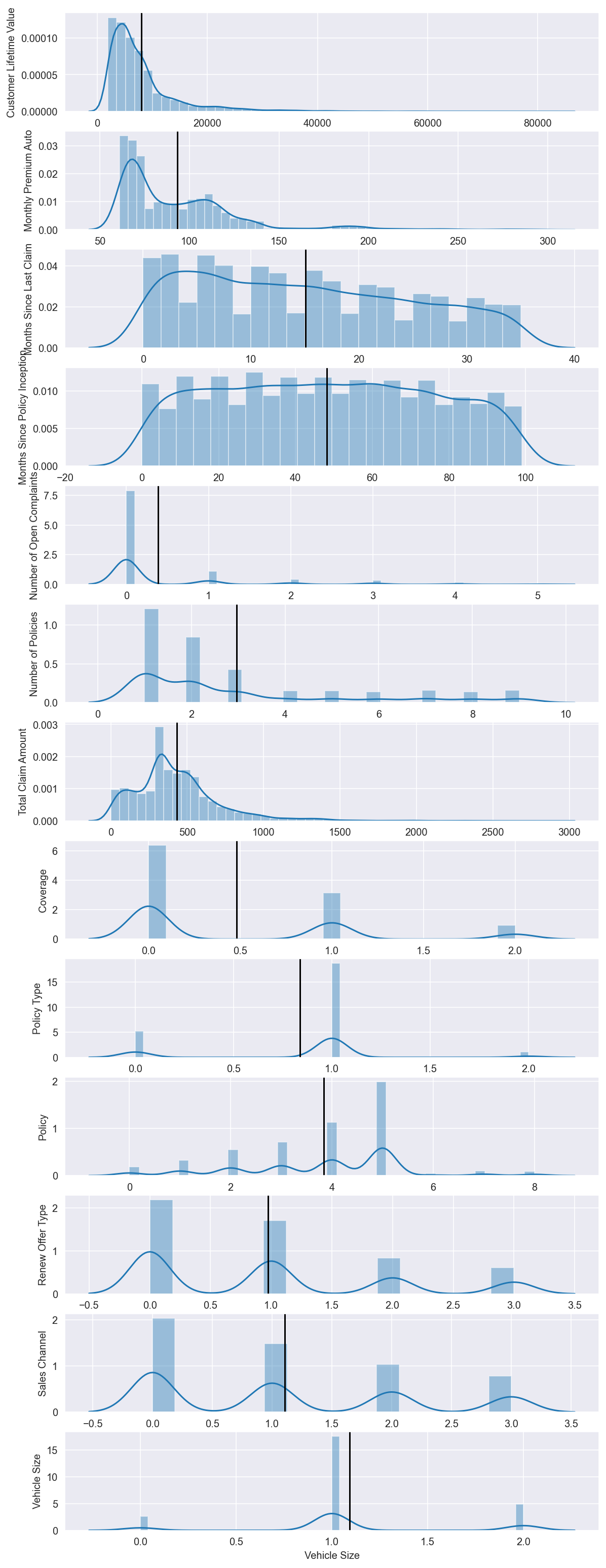
Analyzing the variables for clustering
num = clustering_raw_data.select_dtypes(include=np.number)  # Get numeric columns
n = num.shape[1]  # Number of cols

fig, axes = plt.subplots(n, 1, figsize=(24/2.54, 70/2.54))  # create subplots with n rows and 1 column

for ax, col in zip(axes, num):  # For each column...
    sns.distplot(num[col], ax=ax)   # Plot histogaerm
    ax.set(ylabel= col)
    ax.axvline(num[col].mean(), c='k')  # Plot mean
Check for Correlation in the data
plt.figure(figsize=(10,8))
sns.heatmap(clustering_raw_data.corr(),
            annot=True,
            linewidths=.5,
            center=0,
            cbar=False,
            cmap="YlGnBu")
plt.show()
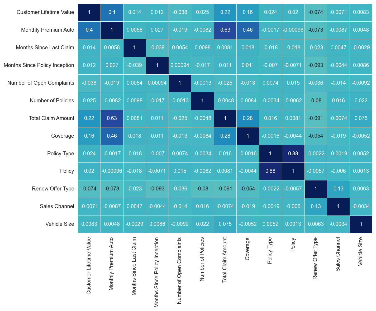
### List columns that can be dropped
columns_drop = ['Policy Type', 'Vehicle Size']
Final data for Clustering after removing unnecessary variables
clustering_raw_data.drop(columns=columns_drop, inplace = True)
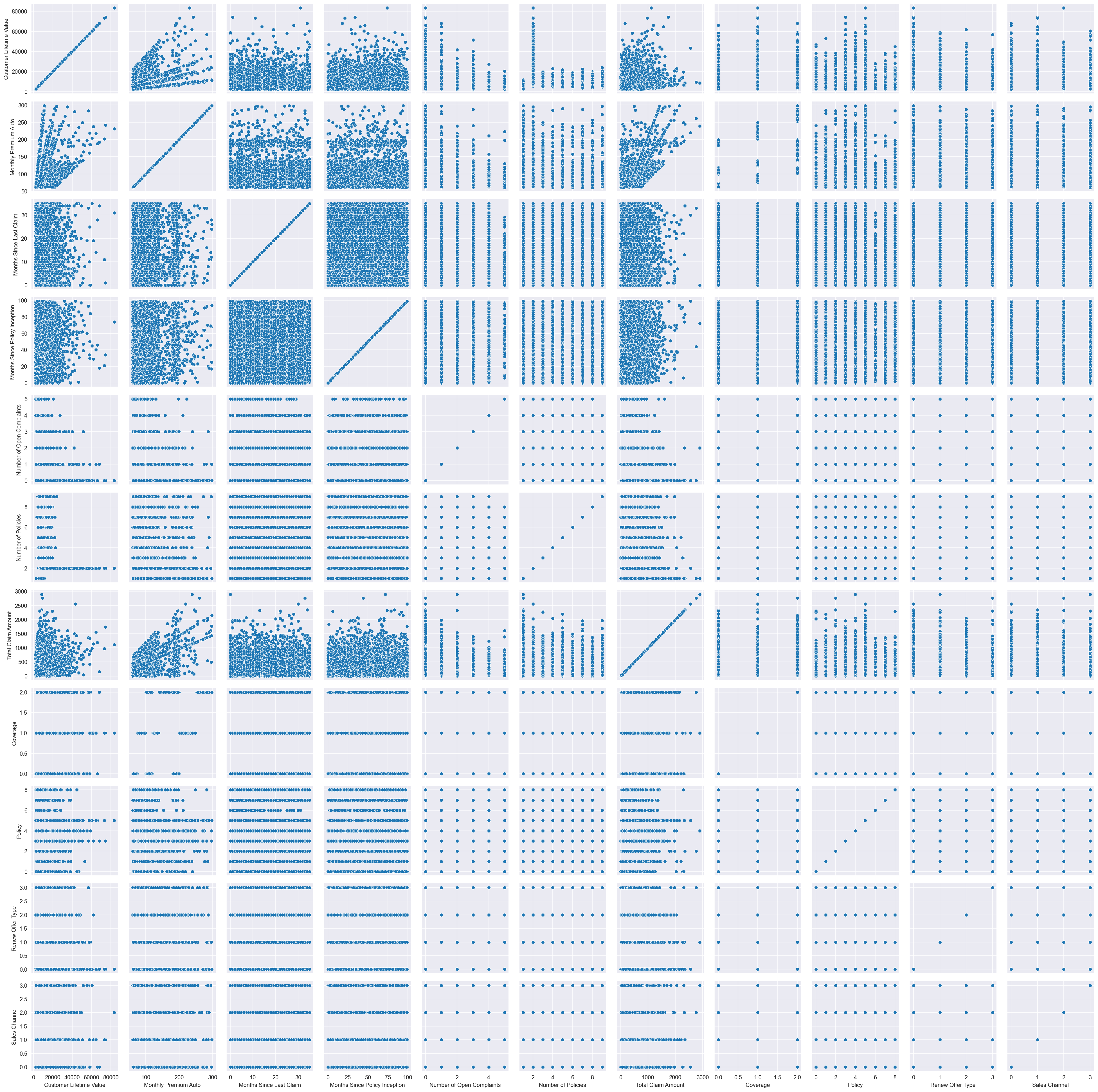
Scatter Plot
g = sns.PairGrid(clustering_raw_data)
g.map(sns.scatterplot);
Standardization
scaler = StandardScaler()
scaled_df = scaler.fit_transform(clustering_raw_data)
scaled_df
array([[-0.76206445, -0.70219428,  1.67841106, ..., -1.14631002,
        -0.96307902, -1.03103509],
       [-0.14630573,  0.0249932 , -0.20538206, ...,  0.72219223,
         1.01635938, -1.03103509],
       [ 0.71655576,  0.43221818,  0.29035297, ...,  0.72219223,
        -0.96307902, -1.03103509],
       ...,
       [-0.43243113, -0.87671927,  0.786088  , ...,  0.72219223,
        -0.96307902, -1.03103509],
       [-0.45956231, -0.78945677,  1.57926405, ...,  0.72219223,
         0.02664018,  0.83309108],
       [ 1.40856681, -0.87671927,  1.48011705, ...,  0.72219223,
         0.02664018, -1.03103509]])
Normalization
normalized_df = normalize(scaled_df)
normalized_df = pd.DataFrame(normalized_df)
normalized_df
| 0 | 1 | 2 | 3 | 4 | 5 | 6 | 7 | 8 | 9 | 10 | |
|---|---|---|---|---|---|---|---|---|---|---|---|
| 0 | -0.229530 | -0.211497 | 0.505529 | -0.467190 | -0.128236 | -0.247465 | -0.049014 | -0.221104 | -0.345263 | -0.290075 | -0.310543 |
| 1 | -0.039185 | 0.006694 | -0.055008 | -0.059191 | -0.114032 | 0.564325 | 0.653961 | 0.212106 | 0.193427 | 0.272214 | -0.276145 |
| 2 | 0.234110 | 0.141212 | 0.094863 | -0.119184 | -0.139102 | -0.131744 | 0.153857 | 0.757311 | 0.235951 | -0.314652 | -0.336855 |
| 3 | -0.016298 | 0.124442 | 0.096599 | 0.201558 | -0.141648 | 0.561799 | 0.114211 | -0.244228 | -0.588586 | -0.320412 | 0.277166 |
| 4 | -0.315172 | -0.244644 | -0.127169 | -0.062264 | -0.177793 | -0.343099 | -0.427272 | -0.306550 | -0.218600 | -0.402175 | -0.430553 |
| ... | ... | ... | ... | ... | ... | ... | ... | ... | ... | ... | ... |
| 8094 | 0.118296 | -0.177388 | -0.601452 | -0.319447 | -0.197588 | -0.187136 | 0.140186 | 0.367524 | 0.335158 | 0.012363 | 0.386624 |
| 8095 | 0.008330 | 0.264696 | 0.187942 | -0.106637 | -0.205438 | 0.612927 | 0.012367 | -0.354214 | 0.348474 | -0.464707 | -0.047756 |
| 8096 | -0.173029 | -0.350802 | 0.314537 | -0.318578 | -0.170359 | 0.006056 | -0.359218 | -0.293731 | 0.288971 | -0.385357 | -0.412548 |
| 8097 | -0.095778 | -0.164531 | 0.329136 | 0.156231 | 0.823254 | 0.264735 | -0.083356 | -0.152992 | 0.150513 | 0.005552 | 0.173625 |
| 8098 | 0.465841 | -0.289948 | 0.489504 | -0.358428 | -0.140807 | -0.133359 | -0.246763 | -0.242778 | 0.238843 | 0.008810 | -0.340984 |
8099 rows × 11 columns
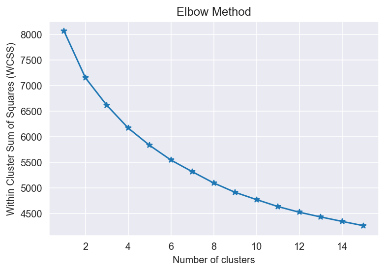
K Means Loop
### The Elbow Method

sse = {}

for k in range(1, 16):
    kmeans = KMeans(n_clusters=k, init='k-means++',random_state= 0 ,max_iter=300).fit(normalized_df)
    sse[k] = kmeans.inertia_ # Inertia: Sum of distances of samples to their closest cluster center

    plt.figure()
plt.plot(list(sse.keys()), list(sse.values()),marker='*')
plt.title('Elbow Method')                               # Set plot title
plt.xlabel('Number of clusters')                        # Set x axis name
plt.ylabel('Within Cluster Sum of Squares (WCSS)')
plt.show()
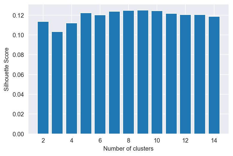
#### The Silhouette Coefficient Method

silhouette_scores = []

for n_cluster in range(2, 15):
    silhouette_scores.append(
        silhouette_score(normalized_df, KMeans(n_clusters = n_cluster).fit_predict(normalized_df)))

# Plotting a bar graph to compare the results
k = [2, 3, 4, 5, 6,7, 8,9, 10,11, 12,13, 14]
plt.bar(k, silhouette_scores)
plt.xlabel('Number of clusters', fontsize = 10)
plt.ylabel('Silhouette Score', fontsize = 10)
plt.show()
Summary of clusters
def cluster_summary(k,norm_data): ## k is no of cluster $ norm_data is normalized data
    final_clusters = KMeans(n_clusters = k).fit_predict(norm_data)
    final_clusters_data = pd.concat([pd.DataFrame(final_clusters),clustering_raw_data],axis=1)
    final_clusters_data.rename(columns={0:"Cluster_Label"}, inplace= True)
    metrics = final_clusters_data.groupby("Cluster_Label").size().reset_index(name = "Distribution")
#     metrics["Perc"] = metrics.groupby("Cluster_Label")["Distribution"].apply(lambda x: x/float(x.sum()))
    metrics["Perc"] = 100*metrics["Distribution"]/metrics["Distribution"].sum()
    return metrics

metrics = cluster_summary(5,normalized_df)
metrics
| Cluster_Label | Distribution | Perc | |
|---|---|---|---|
| 0 | 0 | 2052 | 25.336461 |
| 1 | 1 | 1337 | 16.508211 |
| 2 | 2 | 2107 | 26.015557 |
| 3 | 3 | 1774 | 21.903939 |
| 4 | 4 | 829 | 10.235832 |
kmeans1 = KMeans(n_clusters=5, init='k-means++',random_state= 0 ,max_iter=300).fit(normalized_df)
kmeans1.cluster_centers_
array([[-0.04920795, -0.06141981,  0.02923496, -0.01958611,  0.59769328,
        -0.04056441, -0.05085618, -0.05004137,  0.01505635, -0.0722779 ,
        -0.02862492],
       [ 0.15252393,  0.24578779,  0.0053302 , -0.01923499, -0.08539613,
        -0.08718466,  0.21197069,  0.28563643,  0.0087514 , -0.0690205 ,
        -0.03748331],
       [-0.10595862, -0.17538956, -0.08656241,  0.17939367, -0.131911  ,
        -0.1792572 , -0.13676129, -0.20394053,  0.01390859, -0.18575648,
        -0.21325831],
       [-0.07251267, -0.08624036,  0.00896877, -0.02048995, -0.08638391,
         0.55051008, -0.06158958, -0.06240628,  0.00109123, -0.06119222,
        -0.01139739],
       [-0.1062052 , -0.15340922,  0.03206375, -0.13361091, -0.11164804,
        -0.16096557, -0.13028584, -0.132813  ,  0.00401019,  0.28438093,
         0.2230994 ]])