The New Brunswick Department of Health, Health Analytics branch, fosters the strategic use of information and analytics to inform decision making as it relates to the Department’s mandate of planning, funding and monitoring a high quality & sustainable health system for the citizens of New Brunswick.
Virtual Care Utilization
About the Data
The world of digital health is continuously expanding and has enormous potential to provide adequate, cost-efficient, safe andscalable eHealth interventions to improve health and health care.It is time to reimagine the traditional, in-person approach to care.
Digital health solutions can change the way New Brunswickers receive services and how citizens and providers engage with the health-care system. These services or interventions should bedesigned around the patient’s needs and pertinent informationshould be shared in a proactive and efficient way through smarter use of data, devices, communication platforms and people.
This data set contains an aggregation of patient visits that have occurred during the pandemic. As part of the pandemic response, which includes the new program to support virtual care delivery for the public. The data elements within the data set will allow you to trend the progress of virtual visits, and to describe the characteristics of patients and physicians who have embraced virtual care.The data set contains 113,202 rows including title headers.
import numpy as np
import pandas as pd
import matplotlib.pyplot as plt
import seaborn as sns
from sklearn import linear_model
from sklearn.linear_model import LogisticRegression
from sklearn.model_selection import train_test_split
from sklearn.metrics import classification_report, confusion_matrix

from sklearn.metrics import mean_squared_error
from math import sqrt
import statsmodels.api as sm

import warnings
warnings.filterwarnings("ignore")
C:\Users\Shivam Goyal\anaconda3\lib\site-packages\statsmodels\tsa\base\tsa_model.py:7: FutureWarning: pandas.Int64Index is deprecated and will be removed from pandas in a future version. Use pandas.Index with the appropriate dtype instead.
  from pandas import (to_datetime, Int64Index, DatetimeIndex, Period,
C:\Users\Shivam Goyal\anaconda3\lib\site-packages\statsmodels\tsa\base\tsa_model.py:7: FutureWarning: pandas.Float64Index is deprecated and will be removed from pandas in a future version. Use pandas.Index with the appropriate dtype instead.
  from pandas import (to_datetime, Int64Index, DatetimeIndex, Period,
df.head()
| YYYYMM | Year | Month | Age Group Code (Patient) | Patient Age Group | Age Group (Patient) | Gender (Patient) | Patient Gender | Health Zone (Patient) | Patient Health Zone | Gender (Physician) | Physician Gender | Health Zone (Physician) | Physician Health Zone | Visit Type | Number of Visits | |
|---|---|---|---|---|---|---|---|---|---|---|---|---|---|---|---|---|
| 0 | 202112 | 2021 | 12 | 4 | 0-20 Years | 15 - 19 Years | 1 | Male | 3 | Fredricton Area | 1 | Male | 7 | Miramichi Area | Office | 9103 |
| 1 | 202103 | 2021 | 3 | 4 | 0-20 Years | 15 - 19 Years | 1 | Male | 3 | Fredricton Area | 2 | Female | 1 | Moncton Area | Office | 4591 |
| 2 | 202111 | 2021 | 11 | 4 | 0-20 Years | 15 - 19 Years | 1 | Male | 3 | Fredricton Area | 2 | Female | 1 | Moncton Area | Office | 4448 |
| 3 | 202104 | 2021 | 4 | 4 | 0-20 Years | 15 - 19 Years | 1 | Male | 3 | Fredricton Area | 2 | Female | 1 | Moncton Area | Office | 4435 |
| 4 | 202102 | 2021 | 2 | 4 | 0-20 Years | 15 - 19 Years | 1 | Male | 3 | Fredricton Area | 2 | Female | 1 | Moncton Area | Office | 4370 |
df.columns, len(df.columns)
(Index(['YYYYMM', 'Year', 'Month', 'Age Group Code (Patient)',
        'Patient Age Group', 'Age Group (Patient)', 'Gender (Patient)',
        'Patient Gender', 'Health Zone (Patient)', 'Patient Health Zone',
        'Gender (Physician)', 'Physician Gender', 'Health Zone (Physician)',
        'Physician Health Zone', 'Visit Type', 'Number of Visits'],
       dtype='object'),
 16)
(df.groupby(['Year','Month'])['Number of Visits'].sum().reset_index()).groupby(['Year'])['Number of Visits'].sum().reset_index().mean()
Year                   2020.50
Number of Visits    2436942.75
dtype: float64
(df.groupby(['Year','Patient Gender'])['Number of Visits'].sum().reset_index()).groupby(['Patient Gender'])['Number of Visits'].mean().reset_index()
| Patient Gender | Number of Visits | |
|---|---|---|
| 0 | Female | 1378825.25 |
| 1 | Male | 1058107.50 |
| 2 | Not Specified | 10.00 |
df.groupby(['Year'])['Physician Gender'].count().reset_index()
| Year | Physician Gender | |
|---|---|---|
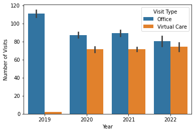
| 0 | 2019 | 22627 |
| 1 | 2020 | 36737 |
| 2 | 2021 | 43025 |
| 3 | 2022 | 10812 |
(df.groupby(['Year','Month'])['Number of Visits'].sum().reset_index()).groupby(['Year'])['Number of Visits'].mean().reset_index().to_csv("Monthly Average Visits.csv")
(df.groupby(['Year','Patient Health Zone'])['Number of Visits'].sum().reset_index()).groupby(['Patient Health Zone'])['Number of Visits'].mean().reset_index()

# .to_csv("Monthly Average Visits.csv")
| Patient Health Zone | Number of Visits | |
|---|---|---|
| 0 | Bathurst Area | 299642.25 |
| 1 | Campbellton Area | 69923.50 |
| 2 | Edmunston Area | 115816.75 |
| 3 | Fredricton Area | 566323.50 |
| 4 | Miramichi Area | 133572.25 |
| 5 | Moncton Area | 627299.75 |
| 6 | Saint John Area | 615620.50 |
| 7 | Unknown | 8744.25 |
# Visits Across Time
pd.pivot_table(df, values='Number of Visits', index=['Year', 'Month'],
                    columns=['Visit Type'], aggfunc=np.sum).reset_index().to_csv("Visitsacrosstime.csv",index = False)
# Visits Across Patient Health Zone
pd.pivot_table(df[(df['Year']==2020) | (df['Year']==2021)],
               values='Number of Visits', index=['Patient Health Zone'],
               columns=['Visit Type'],
               aggfunc=np.sum).reset_index().to_csv("VisitsPatientHealthZone.csv",index = False)
# Visits Across Physician Health Zone
pd.pivot_table(df[(df['Year']==2020) | (df['Year']==2021)],
               values='Number of Visits', index=['Physician Health Zone'],
               columns=['Visit Type'],
               aggfunc=np.sum).reset_index().to_csv("VisitsPhysicianHealthZone.csv",index = False)
# Visits Across Patient Gender
pd.pivot_table(df[(df['Year']==2020) | (df['Year']==2021)],
               values='Number of Visits', index=['Patient Gender'],
               columns=['Visit Type'],
               aggfunc=np.sum).reset_index().to_csv("VisitsPatientGender.csv",index = False)
# Visits Across Physician Gender
pd.pivot_table(df[(df['Year']==2020) | (df['Year']==2021)],
               values='Number of Visits', index=['Physician Gender'],
               columns=['Visit Type'],
               aggfunc=np.sum).reset_index().to_csv("VisitsPhysicianGender.csv",index = False)
# Visits Across Patient Age Group
pd.pivot_table(df[(df['Year']==2020) | (df['Year']==2021)],
               values='Number of Visits', index=['Age Group (Patient)'],
               columns=['Visit Type'],
               aggfunc=np.sum).reset_index().to_csv("VisitsPatientAgeGroup.csv",index = False)
# Visits Across Patient and Physician Health Zone Combined
pd.pivot_table(df[(df['Year']==2020) | (df['Year']==2021)],
               values='Number of Visits', index=['Patient Health Zone','Physician Health Zone'],
               columns=['Visit Type'],
               aggfunc=np.sum).reset_index().to_csv("VisitsPatientPhysicianHealthZone.csv",index = False)
# Visits Across Patient Gender & Health Zone Combined
pd.pivot_table(df[(df['Year']==2020) | (df['Year']==2021)],
               values='Number of Visits', index=['Patient Health Zone','Patient Gender'],
               columns=['Visit Type'],
               aggfunc=np.sum).reset_index().to_csv("patient healthzone gender.csv",index=False)
# Visits Across Physician Gender & Health Zone Combined
pd.pivot_table(df[(df['Year']==2020) | (df['Year']==2021)],
               values='Number of Visits', index=['Physician Health Zone','Physician Gender'],
               columns=['Visit Type'],
               aggfunc=np.sum).reset_index().to_csv("Physician healthzone gender.csv",index=False)
Forecast
Moving Average
# Visits Across Patient and Time
forecast_data = pd.pivot_table(df[~(df['Year']==2022)],
               values='Number of Visits', index=['YYYYMM'],
               columns=['Visit Type'],
               aggfunc=np.sum).reset_index()
forecast_data = forecast_data.loc[:,['YYYYMM','Virtual Care']]
forecast_data
train = forecast_data.iloc[13:,]
train
| Visit Type | YYYYMM | Virtual Care | MA |
|---|---|---|---|
| 13 | 202005 | 73908.0 | NaN |
| 14 | 202006 | 170473.0 | NaN |
| 15 | 202007 | 145645.0 | 130008.666667 |
| 16 | 202008 | 125760.0 | 147292.666667 |
| 17 | 202009 | 144209.0 | 138538.000000 |
| 18 | 202010 | 137580.0 | 135849.666667 |
| 19 | 202011 | 140555.0 | 140781.333333 |
| 20 | 202012 | 133632.0 | 137255.666667 |
| 21 | 202101 | 169229.0 | 147805.333333 |
| 22 | 202102 | 154023.0 | 152294.666667 |
| 23 | 202103 | 165160.0 | 162804.000000 |
| 24 | 202104 | 146006.0 | 155063.000000 |
| 25 | 202105 | 140076.0 | 150414.000000 |
| 26 | 202106 | 144661.0 | 143581.000000 |
| 27 | 202107 | 108489.0 | 131075.333333 |
| 28 | 202108 | 105513.0 | 119554.333333 |
| 29 | 202109 | 124829.0 | 112943.666667 |
| 30 | 202110 | 122944.0 | 117762.000000 |
| 31 | 202111 | 128506.0 | 125426.333333 |
| 32 | 202112 | 115565.0 | 122338.333333 |
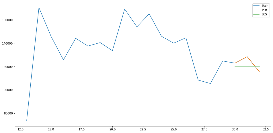
train['MA'] = train['Virtual Care'].rolling(window=2).mean()
rms = sqrt(mean_squared_error(train.loc[30:,'Virtual Care'],train.loc[30:,'MA']))
print(rms)
4102.423572312672
test = train.loc[30:,]
test
| Visit Type | YYYYMM | Virtual Care | MA |
|---|---|---|---|
| 30 | 202110 | 122944.0 | 123886.5 |
| 31 | 202111 | 128506.0 | 125725.0 |
| 32 | 202112 | 115565.0 | 122035.5 |
# 3 --5234.994913153281
# 2 --4102.423572312672
fit2.forecast(7)
array([119851.48, 119851.48, 119851.48, 119851.48, 119851.48, 119851.48,
       119851.48])
Simple Exponential Smoothening
from statsmodels.tsa.api import ExponentialSmoothing, SimpleExpSmoothing, Holt

fit2 = SimpleExpSmoothing(np.asarray(train.loc[30:,'Virtual Care'])).fit(smoothing_level=0.6,optimized=False)
test['SES'] = fit2.forecast(len(test))
plt.figure(figsize=(16,8))
plt.plot(train['Virtual Care'], label='Train')
plt.plot(test['Virtual Care'], label='Test')
plt.plot(test['SES'], label='SES')
plt.legend(loc='best')
plt.show()
Holt’s Winters
# import statsmodels.api as sm
# sm.tsa.seasonal_decompose(train['Virtual Care']).plot()
# result = sm.tsa.stattools.adfuller(train['Virtual Care'])
# plt.show()
sns.barplot(x = 'Year', y = 'Number of Visits', hue = 'Visit Type', data = df)
#print(df.groupby(['Year', 'Visit Type']).mean()['Number of Visits'])
plt.show()
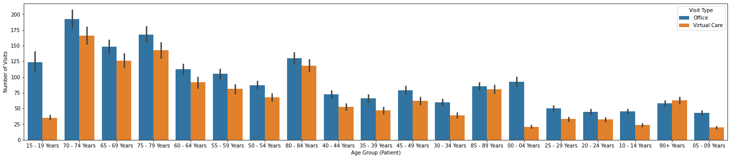
plt.figure(figsize=(25,5))
sns.barplot(x = 'Age Group (Patient)', y = 'Number of Visits', hue = 'Visit Type', data = df)
plt.show()
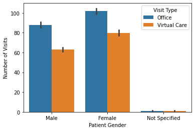
sns.barplot(x = 'Patient Gender', y = 'Number of Visits', hue = 'Visit Type', data = df)
plt.show()
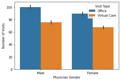
sns.barplot(x = 'Physician Gender', y = 'Number of Visits', hue = 'Visit Type', data = df)
plt.show()
plt.figure(figsize=(25,5))
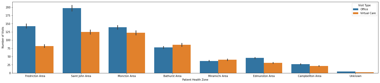
sns.barplot(x = 'Patient Health Zone', y = 'Number of Visits', hue = 'Visit Type', data = df)
plt.show()
plt.figure(figsize=(25,5))
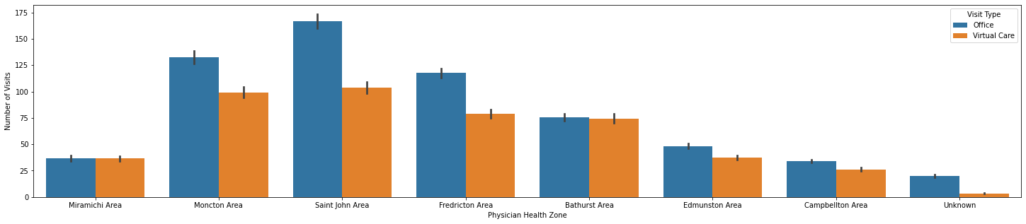
sns.barplot(x = 'Physician Health Zone', y = 'Number of Visits', hue = 'Visit Type', data = df)
plt.show()
Linear Regression Model
dummies=pd.get_dummies(df,drop_first=True)
df=pd.concat([df,dummies.iloc[:,16:46]],axis=1)
#list(dummies.columns)

df_reg=pd.concat([df.iloc[:,0],df.iloc[:,16:46],df.iloc[:,15]],axis=1)
#df_reg=pd.concat([df.iloc[:,0],df.iloc[:,3],df.iloc[:,28:45],df.iloc[:,15]],axis=1)

x=df_reg.loc[:,df_reg.columns!="Number of Visits"]
y=df_reg["Number of Visits"]

x_train, x_test,y_train,y_test = train_test_split(x,y,test_size =0.3)
regr = linear_model.LinearRegression()
regr.fit(x_train, y_train)

#print('Intercept: \n', regr.intercept_)
#print('Coefficients: \n', regr.coef_)

x = sm.add_constant(x_train) # adding a constant

model = sm.OLS(y_train, x_train).fit()
predictions = model.predict(x_test)

print_model = model.summary()
print(print_model)

regr.score(x_test,y_test)
                                 OLS Regression Results
=======================================================================================
Dep. Variable:       Number of Visits   R-squared (uncentered):                   0.218
Model:                            OLS   Adj. R-squared (uncentered):              0.217
Method:                 Least Squares   F-statistic:                              710.9
Date:                Fri, 04 Nov 2022   Prob (F-statistic):                        0.00
Time:                        01:20:15   Log-Likelihood:                     -5.3945e+05
No. Observations:               79240   AIC:                                  1.079e+06
Df Residuals:                   79209   BIC:                                  1.079e+06
Df Model:                          31
Covariance Type:            nonrobust
==========================================================================================================
                                             coef    std err          t      P>|t|      [0.025      0.975]
----------------------------------------------------------------------------------------------------------
Year                                       0.0361      0.002     22.958      0.000       0.033       0.039
Age Group (Patient)_35 - 39 Years         10.6933      3.476      3.076      0.002       3.881      17.506
Age Group (Patient)_40 - 44 Years         15.3216      3.490      4.391      0.000       8.482      22.161
Age Group (Patient)_45 - 49 Years         22.3762      3.482      6.426      0.000      15.552      29.201
Age Group (Patient)_50 - 54 Years         30.1556      3.442      8.761      0.000      23.410      36.902
Age Group (Patient)_55 - 59 Years         48.4215      3.391     14.280      0.000      41.776      55.068
Age Group (Patient)_60 - 64 Years         57.7919      3.349     17.254      0.000      51.227      64.357
Age Group (Patient)_65 - 69 Years         95.5130      3.347     28.534      0.000      88.952     102.074
Age Group (Patient)_70 - 74 Years        134.8046      3.422     39.390      0.000     128.097     141.512
Age Group (Patient)_75 - 79 Years        107.7460      3.646     29.554      0.000     100.600     114.892
Age Group (Patient)_80 - 84 Years         75.6499      3.932     19.237      0.000      67.942      83.358
Age Group (Patient)_85 - 89 Years         31.6560      4.133      7.659      0.000      23.555      39.757
Age Group (Patient)_90+ Years              5.8787      4.565      1.288      0.198      -3.068      14.826
Patient Gender_Male                      -19.8723      1.560    -12.738      0.000     -22.930     -16.815
Patient Gender_Not Specified            -129.7541     42.995     -3.018      0.003    -214.024     -45.484
Patient Health Zone_Campbellton Area     -58.0391      3.421    -16.965      0.000     -64.745     -51.334
Patient Health Zone_Edmunston Area       -39.6609      3.556    -11.155      0.000     -46.630     -32.692
Patient Health Zone_Fredricton Area       27.3165      3.022      9.040      0.000      21.394      33.239
Patient Health Zone_Miramichi Area       -48.5354      3.151    -15.403      0.000     -54.711     -42.359
Patient Health Zone_Moncton Area          39.6895      2.942     13.491      0.000      33.923      45.456
Patient Health Zone_Saint John Area       60.7020      3.258     18.632      0.000      54.316      67.088
Patient Health Zone_Unknown             -102.6974      3.586    -28.637      0.000    -109.726     -95.669
Physician Gender_Male                     10.5345      1.566      6.727      0.000       7.465      13.604
Physician Health Zone_Campbellton Area   -32.0513      3.597     -8.911      0.000     -39.101     -25.002
Physician Health Zone_Edmunston Area     -28.1643      3.739     -7.533      0.000     -35.492     -20.837
Physician Health Zone_Fredricton Area      9.6762      2.993      3.233      0.001       3.810      15.542
Physician Health Zone_Miramichi Area     -54.1623      3.079    -17.592      0.000     -60.197     -48.128
Physician Health Zone_Moncton Area        29.3353      2.826     10.382      0.000      23.797      34.874
Physician Health Zone_Saint John Area     34.7255      3.088     11.247      0.000      28.674      40.777
Physician Health Zone_Unknown            -87.6980      4.727    -18.552      0.000     -96.963     -78.433
Visit Type_Virtual Care                  -28.6571      1.611    -17.792      0.000     -31.814     -25.500
==============================================================================
Omnibus:                    90032.920   Durbin-Watson:                   1.985
Prob(Omnibus):                  0.000   Jarque-Bera (JB):         21699933.674
Skew:                           5.593   Prob(JB):                         0.00
Kurtosis:                      83.295   Cond. No.                     1.12e+05
==============================================================================

Notes:
[1] R² is computed without centering (uncentered) since the model does not contain a constant.
[2] Standard Errors assume that the covariance matrix of the errors is correctly specified.
[3] The condition number is large, 1.12e+05. This might indicate that there are
strong multicollinearity or other numerical problems.


0.11132790904846412